amyehodge.github.io
Hands-on Intro to SQL (Structured Query Language)
This workshop will teach the basics of working with and querying structured data in a database environment. This workshop uses the SQLite plugin for Firefox. We will provide laptops with the correct software for the workshop. If you bring your own machine to the workshop, you must have the software installed in advance.
Contents
- Software and data setup
- Dataset description
- Import data into SQLite
- Relational databases and database design
- Why use relational databases
- Database management systems
- Basic queries, including Unique values and Calculated values
- Filtering
- Missing data
- Sorting
- Order of execution vs order of query
- Aggregation
- Joins
- Data types
- Commenting your queries
- Exporting & saving query results
- Saving queries in SQLite Manager
- Running sqlite3 from the command line
- Real life examples: schema and query
- Resources
Software and data setup
If you are using one of the Library’s laptops, skip this section.
- Download Firefox and install it.
- Download and install the SQLite Manager add on: Menu (the three horizontal lines near the top right corner of Firefox) -> Add-ons -> Search -> SQLite Manager -> Install -> Restart now
- Add SQLite Manager to the menu: Menu -> Customize, then drag the SQLite Manager icon to one of the empty menu squares on the right, Exit Customize
- Download the Portal Database as well as the individual csv files for plots, species, and surveys.
- Open SQLite Manager: Menu -> SQLite Manager
Dataset description
The data we will be using is a time-series for a small mammal community in southern Arizona. This is part of a project studying the effects of rodents and ants on the plant community that has been running for almost 40 years. The rodents are sampled on a series of 24 plots, with different experimental manipulations controlling which rodents are allowed to access which plots.
This is a real dataset that has been used in over 100 publications. We’ve simplified it a little bit for the workshop, but you can download the full dataset and work with it using exactly the same tools we’ll learn about today.
CHALLENGE 1
Open each of the csv files and explore them. What information is contained in each file? If you had the following research questions:
- How many specimens of each species were captured in each type of plot?
- What are the minimum, maximum, and average weight for each species of rodent?
- What is the average weight of each rodent species over the course of the years? Is there any noticeable trend for any of the species?
What would you need to answer these questions? Which files have the data you would need? What operations would you need to perform if you were doing these analyses from these csv files?
Import data into SQLite
We can import our data in one of two ways:
- Import the .sqlite database file
- Import the individual tables
Import the .sqlite database file
- Select Database -> Connect Database
- Choose the portal_mammals.sqlite file
Import the individual tables
- Start a New Database by selecting Database -> New Database
- Name your database and save it to the desktop
- Import your data tables into your database by selecting Database -> Import
- Click on the Select File and choose the surveys.csv file
- Give the table a name (or use the default)
- If the the file has column headings in the first row, check the appropriate box (our tables have column headings in the first row)
- Make sure the delimiter and quotation options are correct (our tables use a comma delimiter and double quotes)
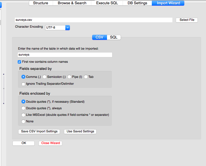
Click OK.
When asked if you want to modify the table, click OK and then set the data types for each column (field) as indicated below.
Data types for each column (field)
| Table | Column | Data Type |
|---|---|---|
| surveys | record_id | integer |
| surveys | month | integer |
| surveys | day | integer |
| surveys | year | integer |
| surveys | plot_id | integer |
| surveys | species_id | text |
| surveys | sex | text |
| surveys | hindfoot_length | real |
| surveys | weight | real |
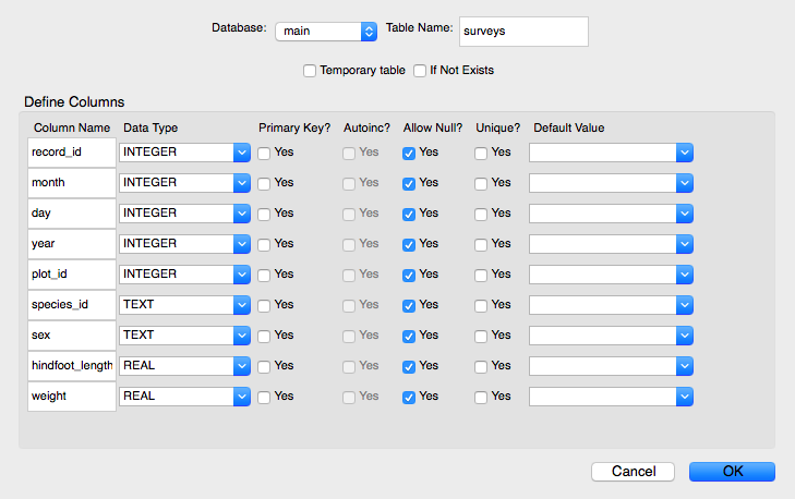
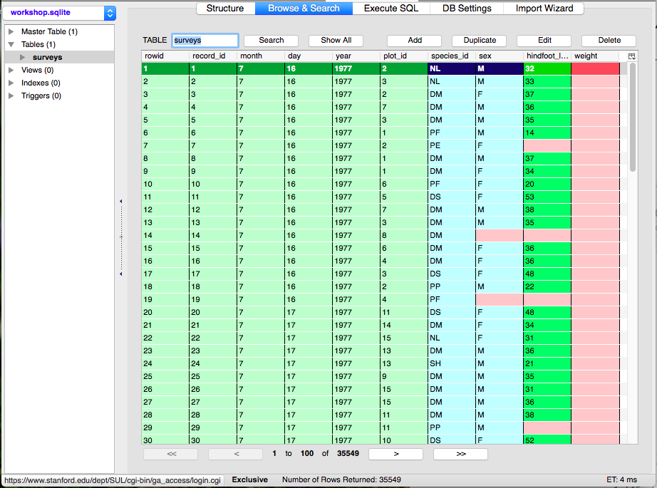
Once the data has been imported, the panel on the left will display a list of the tables under the heading “Tables.”
To see the contents of a table, click on that table and then click on the Browse and search tab in the right hand section of the screen.
CHALLENGE 2
Import the plots and species tables using the information provided in the table below.
| Table | Column | Data Type |
|---|---|---|
| plots | plot_id | integer |
| plots | plot_type | text |
| species | species_id | text |
| species | genus | text |
| species | species | text |
| species | taxa | text |
You can also use this same approach to append new data to an existing table.
Relational databases and database design
- Relational databases store data in tables with fields (columns) and records (rows).
- The records are not in any particular order.
- Data fields have types and all values in a field have the same type (list of data types). We defined these data types when we imported our tables.
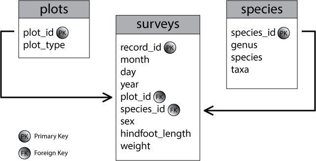
- Each table contains a single field (or combination of fields) that uniquely defines each database record. This field is called the primary key. We defined these as well when we imported our tables.
- Every row-column combination (cell) contains a single atomic value, i.e., not containing parts we might want to work with separately. Note how the genus and species information in the species table are in separate fields.
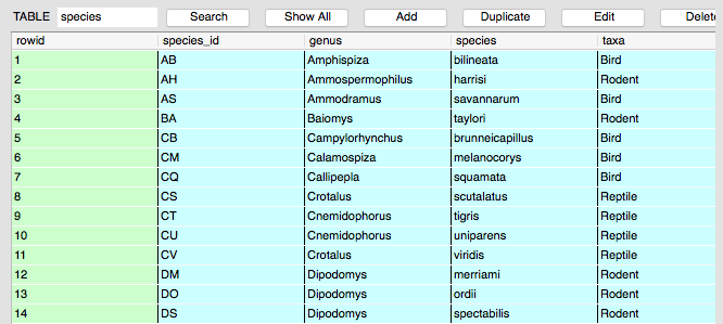
- Data are split into multiple tables, each containing one class of information.
- Tables are related by shared columns of information. The field of data in one table that correlates to the primary key field of another table is called the foreign key.
- Queries let us look up data or make calculations based on the fields of data.
Why use relational databases
- Data separate from analysis.
- There is no risk of accidentally changing data when analyzing it.
- If we change the data we can rerun the query
- It’s fast for large amounts of data.
- It improves quality control of data entry: it’s possible to constrain types, which is especially easy if you use forms available in database programs like Access, Filemaker, etc.
- The concepts of relational database querying are core to understanding how to do similar things using programming languages such as R or Python.
Database management systems
There are a number of different database management systems for working with relational data. We’re going to use SQLite today, but basically everything we teach you will apply to the other database systems as well (e.g., MySQL, PostgreSQL, MS Access, Filemaker Pro). The differences between these are mostly in the details of exactly how to import and export data, the specific data types, and nuances of how the queries are written.
Basic queries
To write a query, click on the Execute SQL tab from within any of your database tables.
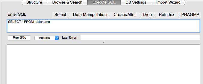
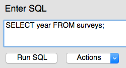
Let’s write a SQL query that selects only the year column from the surveys table. Enter the query in the box labeled “Execute SQL.”
SELECT year FROM surveys;
We have capitalized the words SELECT and FROM because they are SQL keywords. SQL is case insensitive, but capitalizing helps with readability and is good style for SQL. When running queries from the command line or a script file, the queries must end in a semicolon. This is how the software knows this is the end of the query. It’s good practice to get in the habit of doing this, even though this interface does not require it.
To run the query in SQLite, click on the RunSQL button that is underneath the text box. Alternatively, Cmd + ; will also run the query.
If we want more information, we can add a new column to the list of fields, right after SELECT.
SELECT year, month, day FROM surveys;
Or we can return all of the columns in a table using the wildcard “*”.
SELECT * FROM surveys;
CHALLENGE 3
Identify the species ID and weight for each survey item and the date on which it was recorded.
Unique values
If we want only the unique values so that we can quickly see what species have been sampled we use the keyword DISTINCT.
SELECT DISTINCT species_id FROM surveys;
If we choose more than one column, then the distinct pairs of values are returned.
SELECT DISTINCT year, species_id
FROM surveys;
This is a good point to introduce another good style practice for SQL queries. It helps with readability if you separate the parts of the query onto separate lines. So, the above query is better written as:
SELECT DISTINCT year, species_id
FROM surveys;
Calculated values
We can also do calculations with the values in a query. For example, if we wanted to look at the mass of each individual on different dates, but we needed it in kg instead of g we could use this query:
SELECT year, month, day, weight/1000
FROM surveys;
When we run the query, the expression weight/1000 is evaluated for each row and appended to that row, in a new column. Note that if we had used the integer data type for weight and divided by the integer 1000, the results would have been reported as integers. In order to get more significant digits, you would need to include the decimal point (i.e. 1000.0) so that SQL knows you want the results reported as floating point numbers.
Expressions can use any fields, any arithmetic operators (+ - * /) and a variety of built-in functions (MAX, MIN, AVG, SUM, ROUND, UPPER, LOWER, LEN, etc). For example, we could round the values to make them easier to read.
SELECT plot, species_ID, sex, weight, ROUND(weight/1000, 2)
FROM surveys;
CHALLENGE 4
Identify the species ID and weight in milligrams for each survey item and the date on which it was recorded.
Filtering
Databases can also filter data – selecting only the data meeting certain criteria. For example, let’s say we only want data for the species Dipodomys merriami, which has a species code of DM. We need to add a WHERE clause to our query:
SELECT *
FROM surveys
WHERE species_id="DM";
We can do the same thing with numbers. Here, we only want the data since 2000:
SELECT *
FROM surveys
WHERE year >= 2000;
We can use more sophisticated conditions by combining filters with AND as well as OR. For example, suppose we want the data on Dipodomys merriami starting in the year 2000, we can combine those filters using AND.
SELECT *
FROM surveys
WHERE (year >= 2000) AND (species_id = "DM");
Note that the parentheses aren’t needed in this case, but they help with readability.
If we wanted get data for any of the Dipodomys species, which have species IDs of DM, DO, and DS, we can combine those using OR.
	SELECT *
	FROM surveys
	WHERE (species_id = "DM") OR (species_id = "DO") OR (species_id = "DS");
The above query is getting kind of long, so let’s use a shortcut for all those ORs. This time, let’s use IN as one way to make the query easier to understand. IN is equivalent to saying WHERE (species_id = "DM") OR (species_id = "DO") OR (species_id = "DS"), but reads more neatly:
SELECT *
FROM surveys
WHERE species_id IN ("DM", "DO", "DS");
CHALLENGE 5
Produce a table listing the data for all individuals in plot 1 that weighed more than 75 grams, telling us the date, species ID, and weight (in kg).
Continuing with the evaluation of AND and OR, if we wanted to get all the records from before 1980 or from 2000 or later that were about species DM, we might be inclined to write the query this way:
SELECT *
FROM surveys
WHERE year < 1980 OR year >=2000 AND species_id="DM";
However, because AND takes logical precendence over OR, the program will evaluate AND first and then OR, which would give us all records for DM from 2000 or later, combined with all records from before 1980 for any species. The correct way to write this query would be this:
SELECT *
FROM surveys
WHERE (year < 1980 OR year >=2000) AND species_id="DM";
The parentheses ensure that the computer combines AND and OR in the way that we intend.
We started with something simple, then added more clauses one by one, testing their effects as we went along. For complex queries, this is a good strategy to make sure you are getting what you want. It also might be helpful to create a subset of the data that you can easily see in a temporary database to practice your queries on before working on a larger or more complicated database.
CHALLENGE 6
Identify the species ID, weight, and plot ID for each survey item, and include filters so that only individuals caught on plot 1 or plot 2 and that weigh more than 75g are included.
Missing data
NULL can be used in queries to represent missing data (note that NULL is not the same as 0).
For example, to find all instances where the species_id was not entered, we can write this query:
SELECT *
FROM surveys
WHERE species_id IS NULL;
Or to find all cases where a weight value was entered:
SELECT *
FROM surveys
WHERE weight IS NOT NULL;
CHALLENGE 7
Write a query to determine the average weight of the individuals in records 1, 63, and 64. How are
NULLvalues treated?
Sorting
We can also sort the results of our queries by using ORDER BY. Let’s keep going with the query we’ve been writing.
SELECT *
FROM surveys
WHERE (year < 1980 OR year >= 2000) AND (species_id IN ("DM", "DO", "DS"))
ORDER BY plot_id ASC;
The keyword ASC tells us to order it in ascending order. We could alternately use DESC to get descending order.
SELECT *
FROM surveys
WHERE (year < 1980 OR year >= 2000) AND (species_id IN ("DM", "DO", "DS"))
ORDER BY plot_id DESC;
ASC is the default, so you don’t actually need to specify it, but it helps with clarity.
We can also sort on several fields at once. Let’s do by plot and then by species.
SELECT *
FROM surveys
WHERE (year < 1980 OR year >= 2000) AND (species_id IN ("DM", "DO", "DS"))
ORDER BY plot_id ASC, species_id DESC;
CHALLENGE 8
Alphabetize the species table by genus and then species.
Order of execution vs. order of query
We don’t actually have to display a column in our query output in order to use it for sorting that output. For example, let’s say we want to order by the plot ID and species ID, but we only want to see the date, plot, and weight information.
SELECT day, month, year, plot_id, weight
FROM surveys
WHERE year < 1980 AND species_id IN ("DM", "DO", "DS")
ORDER BY plot_id ASC, species_id DESC;
We can do this because sorting occurs earlier in the computational pipeline than field selection.
The computer is basically doing this:
- Collecting data from tables according to
FROM - Filtering rows according to
WHERE - Sorting results according to
ORDER BY - Displaying requested columns or expressions according to
SELECT
When we write queries, SQL dictates the query parts be supplied in a particular order: SELECT, FROM, JOIN...ON, WHERE, GROUP BY, HAVING, ORDER BY. Note that this is not the same order in which the query is executed. (We’ll get to JOIN...ON, GROUP BY, and HAVING in a bit.)
Aggregation
Aggregation allows us to combine results by grouping records based on value and to calculate combined values in groups.
Let’s go to the surveys table and find out how many individuals there are. Using the wildcard counts the number of records (rows).
SELECT COUNT(*)
FROM surveys;
There are many other aggregate functions included in SQL including SUM, MAX, MIN, and AVG. We can find out the average of weight for all of those individuals by using the function AVG.
SELECT COUNT(*), AVG(weight)
FROM surveys;
Something a little more useful might be finding the number and average weight of a particular species in our survey, like DM.
	SELECT COUNT(*), AVG(weight)
FROM surveys
WHERE species_id="DM";
CHALLENGE 9
Calculate the total, average, minimum, and maximum weights of the animals collected over the duration of the survey, then see if you can calculate these values only for animals that weighed between 5 and 10 g.
Now, let’s see how many individuals were counted in each species. We do this using a GROUP BY clause.
SELECT species_id, COUNT(*)
FROM surveys
GROUP BY species_id;
GROUP BY tells SQL what field or fields we want to use to aggregate the data. If we want to GROUP BY by multiple fields, we give GROUP BY a comma separated list.
CHALLENGE 10
- Identify how many animals were counted in each year total.
- Identify how many animals were counted in each year per species.
- Identify the average weight of each species in each year.
- Now try to combine the above queries to list how many and the average weight for each species in each year.
We saw earlier that WHERE allows us to filter results according to some criteria. We can filter results based on aggregate functions as well, using the keyword HAVING.
For example, we can adapt the last query we wrote to only return information about species with a count higher than 10:
	SELECT species_id, COUNT(*)
	FROM surveys
	GROUP BY species_id
	HAVING COUNT(*)>10;
CHALLENGE 11
Figure out how many different genera (that’s the plural of genus!) there are in each taxa, but only for cases where there are 10 or more genera. List the taxa with the most genera at the top.
Joins
To combine data from two tables we use the SQL JOIN command, which comes after the FROM command.
We will also need to use the keyword ON to tell the computer which columns provide the link (Primary Key > Foreign Key) between the two tables. In this case, the species_id column in the species table is defined as the primary key. It contains the same data as the survey table’s species_id column, which is the foreign key in this case. We want to join the tables on these species_id fields.
	SELECT *
	FROM surveys
	JOIN species
	ON surveys.species_id = species.species_id
ON is kind of like WHERE, in that it filters things out according to a test condition. We use the table.colname format to tell the software what column in which table we are referring to.
Field names that are identical in both tables can confuse the software so you must specify which table you are talking about, any time you mention these fields. You do this by inserting the table name in front of the field name as table.colname, as I have done above in the SELECT and GROUP BY parts of the query.
We often won’t want all of the fields from both tables, so anywhere we would have used a field name in a query on a single table, we can use table.colname in our JOIN.
For example, what if we wanted information on when individuals of each species were captured, but instead of their species ID, we wanted their actual species names.
	SELECT surveys.year, surveys.month, surveys.day, species.genus, species.species
	FROM surveys
	JOIN species
	ON surveys.species_id = species.species_id;
CHALLENGE 12
Identify the genus, species, and weight of every individual captured at the site.
We can count the number of records returned by our original JOIN query.
	SELECT COUNT(*)
	FROM surveys
	JOIN species
	ON surveys.species_id = species.species_id
Notice that this number is smaller than the number of records present in the survey data.
This is because, by default, SQL only returns records where the joining value is present in the JOIN columns of both tables (i.e. it takes the intersection of the two JOIN columns). This joining behavior is known as an INNER JOIN (this term can be used interchangeably with JOIN).
We can also tell the computer that we wish to keep all the records in the first table by using the command LEFT OUTER JOIN or LEFT JOIN for short.
CHALLENGE 13
Rewrite the
JOINabove to keep all the entries present in the surveys table. How many records are returned by this query?
Joins can also be combined with sorting, filtering, and aggregation. So, if we wanted average mass of the individuals on each different type of treatment, we could do something like
	SELECT plots.plot_type, AVG(surveys.weight)
	FROM surveys
	JOIN plots
	ON surveys.plot_id = plots.plot_id
	GROUP BY plots.plot_type;
CHALLENGE 14
How many of each genus were caught in each plot? Report the answer with the greatest number at the top of the list.
You can also combine many tables using a JOIN. The query must include enough JOIN…ON clauses to link all of the tables together. In the query below, we are now looking at the count of each species for each type of plot during each year. This required 1) adding in an extra JOIN…ON clause, 2) including plot_type in the SELECT portion of the statement, and 3) adding plot_type to the GROUP BY function:
SELECT surveys.species_id, surveys.year, plots.plot_type, COUNT(*), surveys.AVG(weight)
FROM surveys
JOIN species ON surveys.species_id = species.species_id
JOIN plots ON plots.plot_id = surveys.plot_id
GROUP BY surveys.species_id, year, plot_type
ORDER BY COUNT(*) DESC;
CHALLENGE 15
SQL queries help us ask specific questions which we want to answer about our data. The real skill with SQL is to know how to translate our scientific questions into a sensible SQL query (and subsequently visualize and interpret our results).
Have a look at the following questions; these questions are written in plain English. Can you translate them to SQL queries and give a suitable answer?
- How many plots of each treatment type are there?
- How many male and female specimens were identified each year? We aren’t interested in cases where the sex is not known.
- How many specimens of each species were captured in each type of plot? We aren’t interested if the species isn’t known.
- What is the average weight of each taxa?
- What are the minimum, maximum, and average weight for each species of rodent?
- What is the average hindfoot length for male and female rodent of each species? Is there a male/female difference?
- What is the average weight of each rodent species over the course of the years? Is there any noticeable trend for any of the species?
- What is the percentage of each species in each taxa? (Hint: Start by determining how many of each species there are in each taxa and then see if you can figure out how to report the percentages. Why do the numbers not add up to 100%?)
Data types
The following table shows some common SQL data types. Different database platforms may have slightly different data types.
| Data type | Description |
|---|---|
| CHARACTER(n) | Character string. Fixed-length n |
| VARCHAR(n) or CHARACTER VARYING(n) | Character string. Variable length. Maximum length n |
| BINARY(n) | Binary string (0s and 1s). Fixed-length n |
| BOOLEAN | Stores TRUE or FALSE values |
| VARBINARY(n) or BINARY VARYING(n) | Binary string. Variable length. Maximum length n |
| INTEGER(p) | Integer numerical (no decimal). Precision p. |
| SMALLINT | Integer numerical (no decimal). Precision 5. |
| INTEGER | Integer numerical (no decimal). Precision 10. |
| BIGINT | Integer numerical (no decimal). Precision 19. |
| DECIMAL(p,s) | Exact numerical, precision p, scale s. Example: decimal(5,2) is a number that has 3 digits before the decimal and 2 digits after the decimal |
| NUMERIC(p,s) | Exact numerical, precision p, scale s. (Same as DECIMAL) |
| FLOAT(p) | Approximate numerical, mantissa precision p. A floating number in base 10 exponential notation. The size argument for this type consists of a single number specifying the minimum precision. |
| REAL | Approximate numerical, mantissa precision 7. |
| FLOAT | Approximate numerical, mantissa precision 16. |
| DOUBLE PRECISION | Approximate numerical, mantissa precision 16. |
| DATE | Stores year, month, and day values |
| TIME | Stores hour, minute, and second values |
| TIMESTAMP | Stores year, month, day, hour, minute, and second values |
| INTERVAL | Composed of a number of integer fields, representing a period of time, depending on the type of interval |
| ARRAY | A set-length and ordered collection of elements |
| MULTISET | A variable-length and unordered collection of elements |
| XML | Stores XML data |
Table source: W3 Schools
Commenting your queries
It is good practice to include comments in your queries so that you remember the purpose of the query and other people can understand it’s purpose, and to describe what various parts of the query are doing or why they were included.
Comments are ignored by the software and can be added in one of two ways.
Short comments can be added by including them after two consecutive dashes. A line return signals the end of the comment. In the query below, the comment “– only data from plots 1 & 2” in the 7th line will be ignored. These comments can also included on separate lines.
SELECT species.genus,
	species.species,
	COUNT(*),
	AVG(surveys.weight)
	FROM surveys
JOIN species ON surveys.species_id=species.species_id
	WHERE (surveys.plot=1 OR surveys.plot=2) AND (surveys.weight > 75) -- only data from plots 1 & 2
	GROUP BY species.species_id
	ORDER BY species.species_id;
Longer comments can be added and separated from the query text by enclosing them in a forward slash and asterisk combination (/*...*/), as shown below. These comments can be written on multiple lines and the final asterisk-forward slash combination signals the end of the comment.
	SELECT species.genus,
		species.species,
	COUNT(*),
	AVG(surveys.weight)
	FROM surveys
	JOIN species ON surveys.species_id=species.species_id
	WHERE (surveys.plot=1 OR surveys.plot=2) AND (surveys.weight > 75)
	GROUP BY species.species_id
/* I am grouping the results by species_id because I want to see
	average weights and
total numbers
	separated out for the individual species*/
ORDER BY p.species_id;
Details about commenting code can be found in the SQLite documentation.
Exporting & saving query results
- Export Results: To export your results into a saved file on your computer, click on the button next to Actions and choose Save Result to File. This file is not queryable.
- Save Results: To save your results as a special kind of table called a view, click on View in the main menu and choose Create View. You can view and query this special table in SQLite.
Saving queries in SQLite Manager
It is possible to save queries within the SQLite Manager so that you can run them again later. The program creates a table where the queries are stored. Here are the steps for doing this.
Start by selecting Tools > Use Table for Extension Data
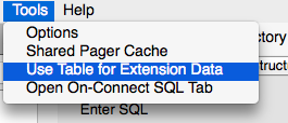
This creates a table in your database called __sm_ext_mgmt and adds new options above and below the Enter SQL box in the Execute SQL tab.
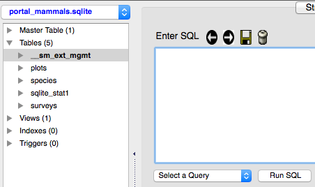
The buttons above the box allow you to scroll forward and backward through your saved queries, to save the current query in the Enter SQL box, and to delete the history of the queries that you have run (this does not delete the queries). Below the box is a drop-down menu that lets you choose a saved query to run.
To save a query, first enter the query in the box.
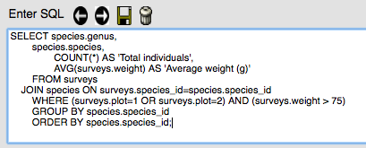
Click on the symbol of the disk (next to the trash can) to save the query. Enter a name for the query in the pop-up box and click OK.
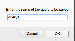
The query is now saved!
When you want to run the query again, select the query from the Select a Query drop-down box.

The query will appear in the Enter SQL box and can be edited before running if desired. Editing the query here will not change the saved query.
To delete a query, run the following statement from the Enter SQL box, replacing “query_name” with the name of your query.
DELETE FROM __sm_ext_mgmt WHERE type="NamedQuery:query_name"
Running sqlite3 from the command line
The SQLite Manager plug in we have been using for this lesson is a convenient interface for working with a database. However, you might want to store and edit queries in a file, or be able to automatically direct your output to a file. These are tasks are much simpler when run from the command line.
SQLite3 can be run directly from the command line. Detailed information about how to do this is available at sqlite.org.
In order to do this you need to be in the shell (Terminal window on Mac), and you need to be in the directory where your .sqlite database file resides. Then just type sqlite3 followed by the name of the .sqlite databases file and you are instantly in the sql interface, ready to type in a query.
Type .help at the prompt to see options available, or check out the more detailed explanation of most of your choices at the sqlite.org link above.
Type .tables to see a list of all your database tables.
Type any SELECT statement directly from the prompt. Be sure to end with a semicolon. That’s how the computer knows you are at the end of the query. Hit Enter or Return after the semicolon to run the query.
Run a query from a .sql file (your query saved as a text document with a .sql file extension) by typing .read followed by a space and the file name.
Type .mode csv to change the standard output to .csv format (instead of delimited by pipes).
Type .once followed by a space and a file name to send the output from the next .read query to a file instead of to the screen.
Type .exit to leave sqlite.
Real life examples
Database schema
The image below is an example of a database schema for an actual database - CyBase. Cybase is a database of cyclic proteins that contains information about proteins, structures, and assays.
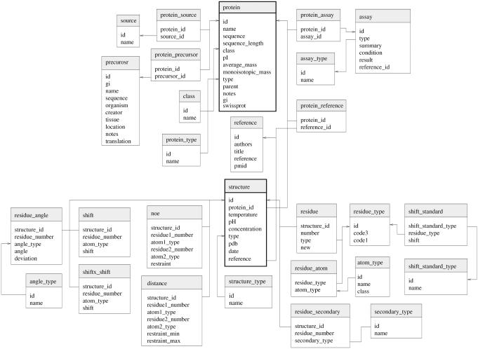
Schema source:
Mulvenna, Jason P.; Wang, Conan; Craik, David J. (2011): Schematic of the relational database underlying CyBase. figshare. http://dx.doi.org/10.6084/m9.figshare.6775 Retrieved 17:23, Sep 16, 2015 (GMT)
SQL query
This is an actual query used in an analysis of Twitter data. The goal of the research was to “validate Twitter as a real-time content, sentiment, and public attention trend-tracking tool” to measure public perceptions in emergencies. In this case they were looking specifically at swine flu. This query is also available in a text file. See the source listed below the query for all the SQL queries used in this research (note how their non-standard formatting is really hard to read!).
See if you can understand how this query works, even without the database tables. We covered all of this in our lesson!
SELECT
	DISTINCT T.title, T.tweetid, T.id, T.publishdate, T.link, T.content, T.updatedate, T.authorname,
	T.authoruri, W.webcite_id, W.long_url,
	COUNT( T.title ) AS number_hits
FROM tweets T
LEFT JOIN webcite W ON T.tweetid = W.tweetid
WHERE
	publishdate BETWEEN "2009-05-01 00:00:00" AND "2009- 12-31 23:59:59"
	AND
 		((LOWER(`title`) LIKE "%swine flu%" OR LOWER(`title`) LIKE "%swineflu%" OR
	LOWER(`title`) LIKE "%h1n1%"))
 		AND
 		((LOWER(`title`) NOT LIKE "%rt @%"
 		AND
 		LOWER(`title`) NOT LIKE "%rt@%"))
 		AND
 		((LOWER(title) LIKE "%http://%") OR (LOWER(title) LIKE "%https://%"))
 	GROUP by title
 	ORDER BY publishdate ASC;
Query source:
SQL Queries for Automated Tweet Coding & Analysis. SQL syntax for search patterns and keywords used by Infovigil for automated tweet coding and analysis.
doi:10.1371/journal.pone.0014118.s001
Resources
- SQL Cheat Sheet
- Challenge Answer Key
- Online tutorials
- W3 Schools
- SQLZOO
- Codecademy
- lynda.com training (free to everyone at Stanford!)
- TutorialsPoint
- Or try some of the tutorials listed here.